Test case - \(\mathrm{LiFeSO_4F}\)#
Here, we use M3GNet to search for low energy \(\ce{LiFeSO4F}\) structures. The DFT results have been previously published here: https://aip.scitation.org/doi/full/10.1063/5.0076220.
The search for \(\ce{LiFeSO4F}\) is more challenging, because the Materials Project database does not have extensive data on the low energy polymorphs. In the work above, we have found several new polymorphs which are not present in the Materials Project database.
## Loading data
lifeso4f_mp = Structure.from_file("LiFeSO4F-mp-943492.vasp")
lifeso4f_mp_relaxed = read("exp-m3gnet/LiFeSO4F-mp-943492.res")
lifeso4f_mp_relaxed_energy = lifeso4f_mp_relaxed.info['energy']  / len(lifeso4f_mp_relaxed)
lifeso4f_mp_relaxed_volume = lifeso4f_mp_relaxed.get_volume() / len(lifeso4f_mp_relaxed)
Energy - Volume distribution#
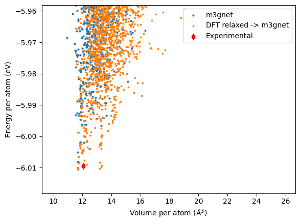
Similar to the \(\ce{LiFePO4}\), we plot the energy per atom against the volume per atom.


Top structure found in each case are shown below. In this case, the M3GNet gives completely different low energy structures which are different to the experimentally found tavorite structure. This is also shown in the distribution plot above where the orange dots do not overlap with the red diamonds (experimental structure).
| label | energy_per_atom | volume_per_atom | |
|---|---|---|---|
| 622 | 2LiFeSO4F-200804-055229-a4aef3 | -6.008125 | 11.683317 |
| 2286 | 2LiFeSO4F-200804-043547-80a807 | -6.008113 | 11.704279 |
| 2002 | 2LiFeSO4F-200818-200625-fa2e89 | -6.005019 | 11.657444 |
| 474 | 2LiFeSO4F-200804-031846-78332d | -6.001975 | 12.084385 |
| 2784 | 2LiFeSO4F-200819-000200-50146f | -6.001975 | 11.862633 |
On the other hand, re-relaxing the DFT relaxed structure gives different sets low energy structures, one has a volume per atom of about 11.8 \(\mathrm{\AA^3}\) while the other has a volume of about 13.2 \(\mathrm{\AA^3}\).
| label | energy_per_atom | volume_per_atom | |
|---|---|---|---|
| 246 | 2LiFeSO4F-200818-173807-f55f90 | -6.010575 | 11.660858 |
| 2488 | 4LiFeSO4F-200804-093629-270f26 | -6.010425 | 11.663456 |
| 2286 | 2LiFeSO4F-200804-043547-80a807 | -6.010275 | 11.670359 |
| 301 | 2LiFeSO4F-200804-034722-678938 | -6.010187 | 13.186974 |
| 2784 | 2LiFeSO4F-200819-000200-50146f | -6.010144 | 11.676132 |
In fact, the sets of low energy structures with large volumes contains the new polymorphs found in the
DFT search previously.
Structure f55f90 (in df_relaxed_m3g) and a4aef3 in (df_m3g) has almost the same structure but the energies are different by 2 meV and almost identical structures have been found for them separately.
| label | energy_per_atom | volume_per_atom | |
|---|---|---|---|
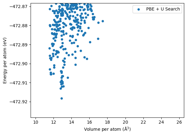
| 301 | 2LiFeSO4F-200804-034722-678938 | -472.918226 | 12.890395 |
| 2434 | 2LiFeSO4F-200804-022644-43b3f4 | -472.913076 | 12.803132 |
| 3860 | 2LiFeSO4F-200804-022154-9da9fb | -472.912053 | 12.918566 |
Energy distribution of the relaxed structures#
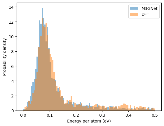
M3GNet seems to give an energy distribution among the relaxed structure very similar to that of the DFT.

Discussion#
Search using M3GNet for relaxation is not able to fully reproduce the DFT results,
and it tends to find a cluster of structure with smaller volumes.
On the other hand, M3GNet does give a reasonable good description for the low energy structures.
In particular, the DFT lowest energy structure 678938 is also found to be one of the lowest energy structure when
the DFT relaxed structure is further relaxed using M£GNet.
This suggests that M3GNet does well when interpolating - even if there are little \(\ce{LiFeSO4F}\) data in the training set,
there are plenty of training data in the composition space of Li-Fe-S-O-F.
