Test case - \(\mathrm{LiN_2}\)#
In this example, we search for \(\ce{LiN2}\) using both DFT and M3GNet. The DFT search is performed first using AIRSS, the M3GNet is used to relax the initial structures and the DFT relaxed structures.
This compound, \(\ce{LiN2}\) has not been reported experimentally, and there is no entry of such stoichiometry in the Materials Project database (as of March 2023).
Load calculated data from files
Energy - Volume distribution#
Similar to the other two cases, we plot the energy per atom against the volume per atom.
Distribution from the M3GNet search is shown below.
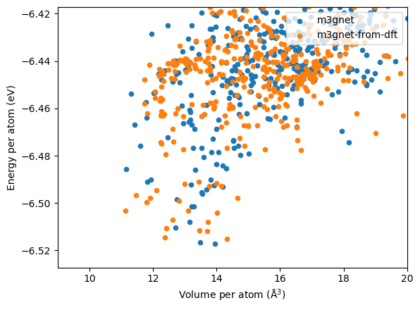
Distribution from the DFT search, which is shown below, is quite different from that of the M3GNet.
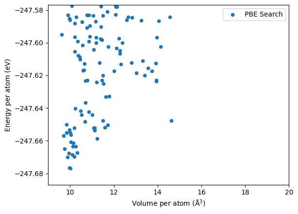
In addition, the lowest energy structure have very different volumes, as the lowest energy structures from the M3GNet are:
| label | energy_per_atom | volume_per_atom | |
|---|---|---|---|
| 763 | LiN2-230326-191233-0e0121 | -247.676850 | 10.018594 |
| 332 | LiN2-230326-180500-a04451 | -247.676533 | 9.974320 |
| 578 | LiN2-230326-200436-4cafc9 | -247.670041 | 9.878006 |
| 90 | LiN2-230326-160120-ac1474 | -247.669627 | 10.188278 |
| 367 | LiN2-230326-195109-76ec78 | -247.668575 | 10.101256 |
| 715 | LiN2-230326-172214-daf21e | -247.667769 | 9.952535 |
| 776 | LiN2-230326-165501-91a048 | -247.667251 | 10.316344 |
| 240 | LiN2-230326-165849-8e77e6 | -247.664903 | 9.740608 |
| 635 | LiN2-230326-180331-4c8ad0 | -247.663535 | 10.266151 |
| 489 | LiN2-230326-202717-e1d113 | -247.663463 | 10.134164 |
and those from the DFT search are:
| label | energy_per_atom | volume_per_atom | |
|---|---|---|---|
| 201 | LiN2-230326-184413-7bd336 | -6.517156 | 13.959285 |
| 344 | LiN2-230326-194612-54678e | -6.516489 | 13.486355 |
| 35 | LiN2-230326-185417-30decd | -6.510256 | 12.715951 |
| 629 | LiN2-230326-151732-ed7287 | -6.507967 | 13.146295 |
| 413 | LiN2-230326-191822-1eaa5a | -6.501428 | 13.276553 |
| 95 | LiN2-230326-170219-f3310a | -6.501311 | 13.219201 |
| 43 | LiN2-230326-180810-1488c9 | -6.498283 | 12.757617 |
| 85 | LiN2-230326-193557-34602e | -6.496022 | 13.555939 |
| 22 | LiN2-230326-180157-b8e352 | -6.495544 | 13.518432 |
| 204 | LiN2-230326-170249-1247e3 | -6.494133 | 13.682473 |
Checking the lowest energy structures visually, we found:
M3GNet relaxed structures feature azide ions, while the DFT ones contains the N2 dimers.
M3GNet relaxed structure are generally high in volume compared to the DFT results.
Energy distribution of the relaxed structures#
The distributions from the two searches are very different, as shown below:
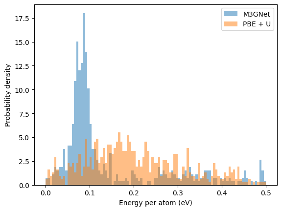
Clearly, this case the M3GNet does not reproduce the PES of the DFT at all, since the two distributions are vastly different. It may appear that M3GNet has a high concentration of low energy structure, this only is due to the reference energy is taken from the lowest energy structure using the same methodology.
Which approach finds lower energy structure?#
It is not possible to compare the energies directly as the DFT calculations are done with CASTEP+QC5 while the M3GNet is trained on VASP+PBE, and unlike previous two cases, we cannot use known lowest structures as references for comparison. The QC5 pseudopotentials used in the search are not designed to be highly transferable but focus on the speed instead. Hence, we re-relax the structures generated from both approaches using CASTEP+C19 at 800 eV and a kpoint spacing of \(0.05 \times 2\pi \AA^{-1}\). C19 is the default pseudopotential library for CASTEP, which has higher accuracy than the QC5 used for searching, but it requires higher cut off energy. The results are shown in the figure below.
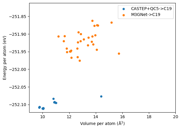
It is clear that the structure from M3GNet are quite high in energy. Relaxing these structures with DFT did change the geometry slightly, but the main structural features remain the same. Clearly, using M3GNet to search for this particularly composition, \(\ce{LiN2}\), would not yield any fruitful results.
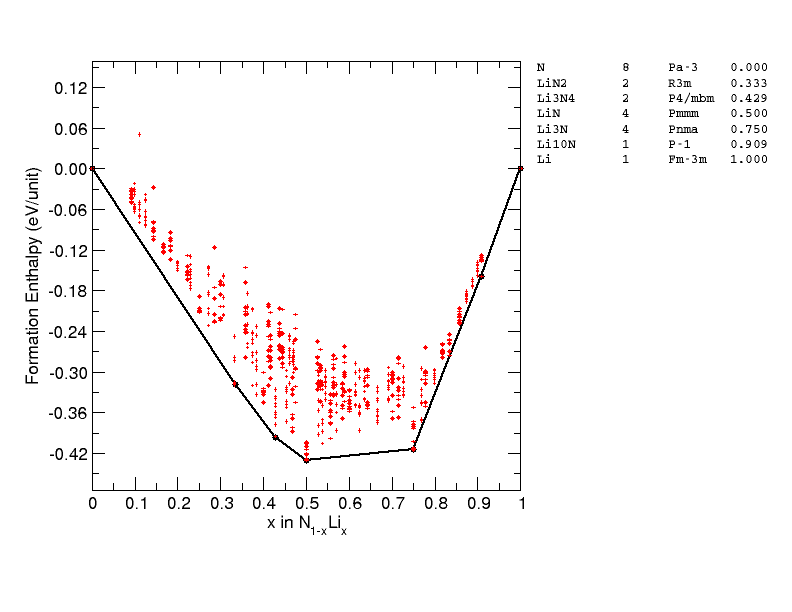
Are the new \(LiN2\) structure found by DFT thermodynamically stable? It turns out the phase diagram of Li-N has indeed been studied previously:
Shen, Y., Oganov, A., Qian, G. et al. Novel lithium-nitrogen compounds at ambient and high pressures. Sci Rep 5, 14204 (2015). https://doi.org/10.1038/srep14204
Where the same \(\ce{LiN2}\) structure has been reported. These structures are not included in the Materials Project dataset, which probably explains why the model does not do well in the Li-N chemical space.
Extras - Machine Learning Potential accelerated search for the Li-N composition space#
Using M3GNet for geometry optimisation would certainly miss the \(\ce{LiN2}\) ground state. This is not surprising because there is no similar structures in the training set.
But can MLPs accelerate AIRSS? A search of Li-N phase space using the recent developed Ephemeral data derived potentials can reproduce the convex hull of Shen et al 2015 above at ambient pressure, but there are also some intriguing new phases found, including \(\ce{Li3N4}\) 🤔🤔.
In this example, the potentials are iteratively built using DFT energies of randomly generated structures. It still at least for now we still need to pay the price of DFT. The training data involves ~ 60k DFT single point energy of small unit cells. This might sound a lot, they are roughly similar to the cost of just 1200 geometry optimisation. The potential built should be able to cover the entire composition space and allow sampling of larger unit cells.
Could one M3GNet make work for the Li-N if these training structures are included in the training? Or perhaps during fine-tuning?
